Tide Analysis
Looking at water level records in coastal waterways, the most obvious clue confirming the presence of the tide is a characteristic, sinusoidal oscillation containing either two main cycles per day (semidiurnal tides), one cycle per day (diurnal tides), or a combination of the two (mixed tides). The underlying principle of tide analysis is that, no matter how complex they may appear, tidal oscillations can be broken down into a collection of simple sinusoids (sinusoids usually represented by the cosine function from trigonometry). Each “cosine” wave will have the same period of oscillation as the celestial forcing that gives rise to it (see Tide Model – Static or Dynamic?). As it turns out, there are quite a few of these.
The purpose of tide analysis is to determine the amplitude and phase (the so-called tidal harmonic constants) of the individual cosine waves, each of which represents a tidal constituent identified by its period in mean solar hours or, alternately, its speed in degrees per mean solar hour (speed = 360°/T where T = period). Finding the tidal harmonic constants at a place allows one to predict tides at that place. Tidal constituent amplitudes are usually given in feet or meters, and phase is usually expressed in degrees. Putting these parts together, the partial tide corresponding to a single tidal constituent is represented by the following equation,
![]()
In this equation, h(t) is the height of the partial tide calculated for time t, and R is the constituent amplitude (equal to one-half the constituent range). The argument for the cosine function includes two terms: Tt , the constituent speed multiplied by time and N, the constituent phase. Notice that the argument could be written as T( t-N ) if we wanted to express the phase in hours instead of degrees. Calculating h for a series of times ranging from 0 to 36 hours yields the following tide graph using R = 1 meter and N = 5 hours:
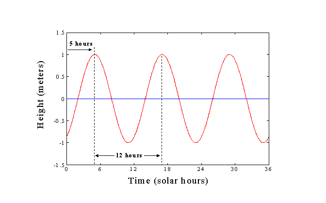
The term phase lag is sometimes used when the phase is expressed in hours as it is in the above example. If the phase had been zero, the cosine wave shown in red would “peak” at the zero hour; Instead, it peaks 5 hours later since N = 5. Although the amplitude and the phase are arbitrary numbers picked for this example, the period of 12 solar hours uniquely identifies this wave as the principal solar semidiurnal constituent with a speed of 30 degrees per mean solar hour. In the jargon of tide analysis, this constituent is represented by the symbol S2 (the subscript “2” means that two of these cycles occur each day).
Suppose the red curve shown above was a record of the actual water level measured at a certain tide station. We wouldn’t really need analysis to come up with the amplitude and phase for a single cosine wave. But what if the curve happened to be the result of several cosine waves added together, all with different amplitude, phase and period. How could we find the amplitude and phase for S2 as well as the other constituents? The answer depends on the length of the record, measurement error, and the analytical technique used but an estimate of the amplitude and phase for any set of tidal constituents whose period we know can be obtained by harmonic analysis, method of least squares (HAMELS). In this method, a set of cosine terms is used as a model. The complete set is made to “fit” the data according to the least squares criterion – simply picking the combination of R and N that causes the sum of the squared differences between observed and model-predicted water levels (calculated, say, at half-hour intervals) to be as small as possible. An easy-to-use HAMELS analysis program is offered to the reader at the end of this tutorial.
BUILDING BLOCKS OF THE TIDE
The following are among the major tidal constituents contributing to the astronomical tide:
M2 - Principal lunar semidiurnal constituent (speed: 28.984 degrees per mean solar hour)
S2 – Principal solar semidiurnal constituent (speed: 30.000 degrees per mean solar hour)
N2 - Larger Lunar elliptic semidiurnal constituent (speed: 28.440 degrees per mean solar hour)
K1 - Luni-solar declinational diurnal constituent (speed: 15.041 degrees per mean solar hour)
O1 - Lunar declinational diurnal constituent (speed: 13.943 degrees per mean solar hour)
M4 - First overtide of M2 constituent (speed: 2 x M2 speed)
M6 - Second overtide of M2 constituent (speed: 3 x M2 speed)
S4 - First overtide of S2 constituent (speed: 2 x S2 speed)
MS4 - A compound tide of M2 and S2 (speed: M2 + S2 speed)
What’s so special about these symbols representing a bunch of squiggly lines? They are literally the building blocks of the tide. The first five constituents are the main players that determine the type of tide that a region experiences. If the amplitudes for M2, S2, and N2 are large compared to the amplitudes for K1 and O1, then tides in the region will be of the semidiurnal type (two highs and two lows each day); if K1 and O1 amplitudes are large compared to the others, then the tides will be of the diurnal type (one high and one low tide each day).
While tidal type stems from amplitude differences among the major tidal constituents, cycles in tidal range (height difference between successive high and low tides) depend on differences in speed. The spring-neap cycle, for example, is due to the speed difference between M2 and S2. S2 is going to complete each 360° cycle a little sooner than M2 because it completes 30° of that cycle in an hour while M2 completes only 28.984°, a speed difference of a little more than a degree per hour. At that rate, S2 will gain on M2 by a full 360° cycle – a spring-neap cycle – every 14 and ¾ days (two cycles every 29 ½ days, a lunar month). As the M2 wave continues to lag behind the S2 wave, the two waveforms pass in and out of phase. We get spring tides when M2 and S2 are in phase so that both waves peak at the same time causing tides of greater range. Neap tides occur when M2 and S2 are out of phase and tend to cancel one another, reducing tidal range. But if you are interested in tides of maximum range, consider what happens when M2, S2, and N2 all peak at about the same time. This results in the so-called perigean-spring tides of maximal range that occur several times a year. Because the tide at any given time is the result of adding a number of different waveforms together, there is always a lot of variation – we shouldn’t expect one spring tide to look exactly like another!
The last four tidal constituents shown above are called shallow-water tides. Tides entering waters where the tidal range is no longer insignificant compared to the depth undergo a transformation that yields additional waves called overtides. Like the “overtones” produced by a musical instrument, the frequency (speed) of an overtide is always an exact multiple of the fundamental frequency – the frequency of the parent wave that underwent transformation. Since their speeds are exact multiples of the parent wave speed, overtides appear fixed or “phase-locked” in time series plots– their waveforms do not move relative to the parent waveform. Instead they “deform” the parent wave and give rise to permanent tidal asymmetries; e.g., differences in the duration of a rising tide versus a falling tide (note there is no difference in duration for the simple cosine wave shown above).
In addition to overtides, other tides called compound tides also arise in shallow water. A compound tide (e.g., MS4) results from the shallow-water interaction of its two parent waves (M2 and S2). There are many more shallow-water tidal constituents but the four listed above do a good job of reconstructing the tidal asymmetries and other fine-scaled behavior seen at most locations.
Two Examples from the Middle East
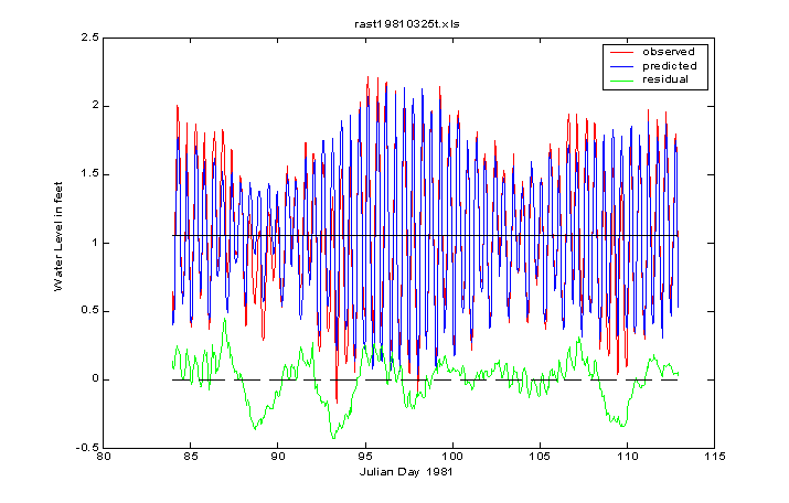
The above graphic depicts a 29-day analysis of a tide record from Ras Tanura, Saudi Arabia. The red curve is the measured water level, the blue curve is the predicted tide based on a tide model using the harmonic constants obtained from the analysis, and the green curve is the residual or the difference between the two. Since the green curve shows some pretty strong deviations from zero, does this mean the predictive model is flawed? Not really. We should expect to see some non-tidal variation in water level showing up in the green curve; in fact, the strongest oscillations that appear there have a period of about 5 days – way longer than tidal. Still, since the analysis used only nine tidal constituents to fit the data, it’s possible that the green curve also contains some minor tidal variation not accounted for in the predictive model. In statistical terms, the tide model appearing above accounts for more than 90 percent of the total variation in water level (r2 = 0.91).
The spring-neap cycle is very apparent at Ras Tanura, a big oil terminal on the west side of the Persian Gulf. The tidal type there is semidiurnal with two highs and two lows each day. But the Persian Gulf (Arabian Gulf to the Saudi Arabs) is a strange place in terms of tidal dynamics. The tide wave entering the Straits of Hormuz generate two large rotary waves for the semidiurnal tide and a single large rotary wave for the diurnal tide inside the Gulf. As you might expect, the amphidromic points for these waves are spaced far apart. To see the consequence of this arrangement on tidal type, look at the next graphic for Safaniya, a coastal town less than two hundred kilometers to the northwest of Ras Tanura.
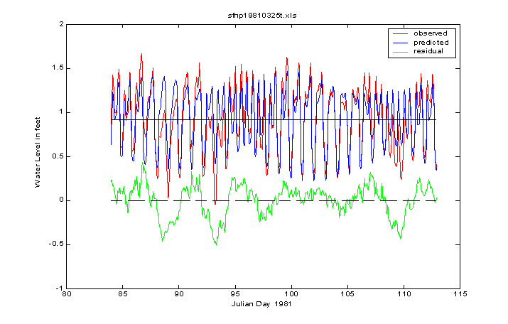
At Safaniya, the tide is mixed, mainly diurnal. In contrast to Ras Tanura, which has a large spring tide on Julian day 97, the tide range is near a minimum on the same day at Safaniya. That’s because the tropic-equatorial cycle takes precedence over the spring-neap cycle at places where the tide type is mainly diurnal. Just as the phasing in-and-out of the principal semidiurnal constituents M2 and S2 produces the spring-neap cycle, the in-and-out phasing of the principal diurnal constituents, K1 and O1, results in the tropic-equatorial cycle.
A quick glance at the residual curve for Safaniya shows that it is almost identical to the one at Ras Tanura. Thus we see that two tide stations with completely different tidal types can experience the same meteorological tide. In fact, the oscillations shown in the green curve coincided with a Shamal, a desert wind that can reach 60 miles per hour and blow for several days, causing periodic water level oscillations in the Northern Persian Gulf basin that last for many more days, like the ringing of a bell.
Note that the range of the astronomical tide at Safaniya is smaller than that at Ras Tanura while the meteorological tide range is about the same at both stations. This is reflected in the percent of total variance accounted for by the tide model, which is only 76 percent (r2 = 0.76) at Safaniya as opposed to 90 percent at Ras Tanura. Clearly the meteorological tide has to be taken into account before evaluating the success of the astronomical tide model!
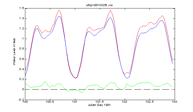
Finally, a place with mixed tides can produce some strange looking curves as the tide transitions from semidiurnal to mixed to diurnal. The following series of daily tides from Safaniya provide a good example:
Now it’s semidiurnal
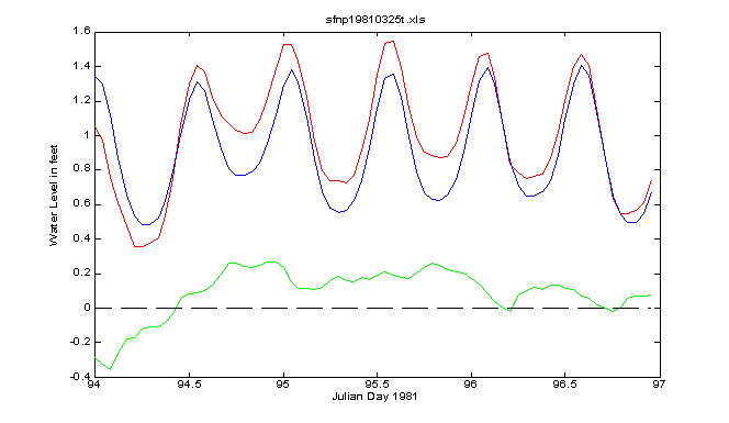
Now it’s mixed
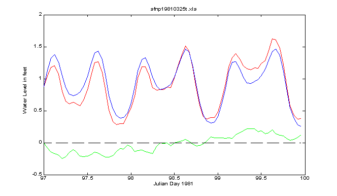
Now it’s diurnal with some strange looking highs
DO YOUR OWN TIDE ANALYSIS - IT’S NOT THAT HARD!
In its infancy, the theory of tides occupied the minds of Europe’s greatest physical scientists in the seventeenth and eighteenth centuries – Newton, LaPlace, Maclaurin, Euler, Bernoulli, among others. Long after the basic principles were put in place by the geniuses of that age, the practical matter of analyzing and predicting sea tides remained something of an art in the hands of a very few. In the days before computers, calculations that we consider simple today represented a huge effort and consequently the task fell to government agencies to perform. Now, at the start of the twenty-first century, a typical desktop computer program requires only five lines of code to derive a set of tidal harmonic constants and very little more to generate tide predictions from these numbers. Yet few of us ever look inside the “black box” since tide prediction tables have always been easy to obtain – the government does these things for us at nominal cost. But if you’re the curious type and even a novice user of MATLAB software by the MathWorks, Inc., a very simple set of programs for tide and tidal current analysis is available at VIMS. You can use these programs to analyze a huge database of water levels and incorporate other data available for free downloading on the NOAA/NOS website: http://co-ops.nos.noaa.gov/. To obtain a copy of the analysis and prediction programs at no cost, please click here and refer to the BOTTOM of that page for information.
