Tidal Current Analysis
First the good news. Currents are analyzed the same way tides are. The same tidal constituents apply and HAMELS (Harmonic Analysis, Method of Least Squares) can again be used to determine the tidal harmonic constants for them. The not-so-good news is that, unlike water level data, water current data are hard to find. This may change soon as new acoustic instrumentation is deployed in more and more places and the data find their way into government and university archives.
We also have a dimensional difference with water currents. Unlike tides, currents can follow any of three spatial dimensions – one vertical and two horizontal. Let’s eliminate the vertical direction to start with. Tidal currents per se involve only horizontal motion. This is clear from their origin, which is firmly linked to the dynamics of long waves (see module on the dynamic model of the tide). And although we could simultaneously analyze water current in two horizontal dimensions – water flow components moving east or west, north or south, for example – it’s usually possible to reduce the dimensionality of the problem to one in coastal waters and inside estuaries. We’ll find out how using water current data from a NOAA/NOS PORTS station near Richmond, California, inside San Francisco Bay.
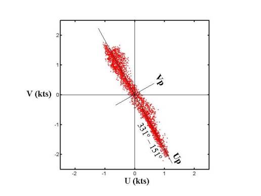
 The practice of using a single dot to show where the tip of
an individual current vector would lie in a U,V plot of many such vectors is explained in the module on current
measurement. The diagram at left shows over three thousand dots representing
orthogonal U,V current components measured
every 6 minutes in a fourteen-day record from Richmond, California. For
example, the lowest dot in the figure represents water flowing east at 1 knot
(U = 1) and south at a little over 2 knots (V = -2.1).
However, if we “freeze” the dots where they are and simply rotate the U,V coordinate axes to a new position, Up,Vp, then almost all of the flow is in the direction of the Up axis. Up is called the principal axis when the flow components projected on to it have the largest possible variance while those projected on to Vp have the least. The orientation of the principal axis shown above is no longer positive east (90° heading) but positive south-southeast (151° heading). An eigenvector algorithm mathematically determines the new orientation but not the heading. You could also go the opposite way and choose a heading of 331° for the positive direction – the Up axis would still retain maximum variance. So which one do you choose? The usual convention is to make the positive coordinate axis coincide with the flood (landward) direction and the negative coordinate axis coincide with the ebb (seaward) direction. Of course, you have to look at the local situation where the current was measured and tell which is the flood direction and which is the ebb. The algorithm has no idea.
Once we settle on a final heading for the flood (positive) axis, another algorithm very quickly carries out the final axis rotation. Going in with a set of current components U and V, we come out with a new set of components, Up and Vp. One of these two is usually loaded with information while the other one isn’t. In the example above, Up accounts for a little more than 99 percent of the total variance in the data. We won’t miss much if we analyze only the Up signal and forget about Vp.
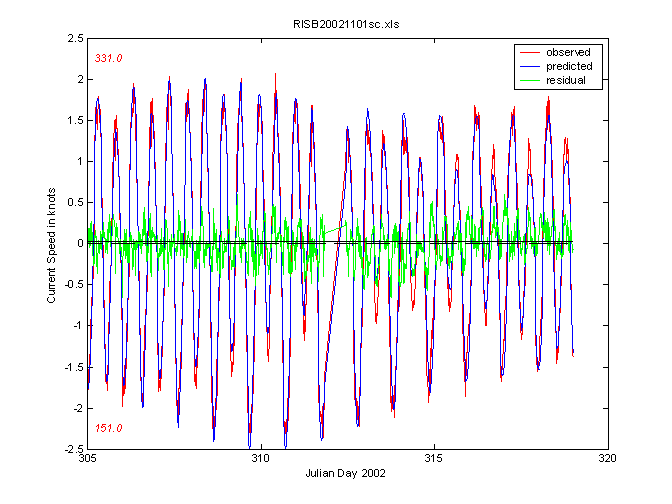
Below is the result of a HAMELS analysis of the Richmond current data starting November 1 (Julian day 305), 2002. This figure is very similar to a tide analysis diagram except that the ordinate is now current speed in knots with positive speeds toward the flood heading of 331° true and negative speeds toward the ebb heading of 151° true. The main oscillations back and forth between flood and ebb once again take the form of the familiar cosine wave - with two floods and two ebbs per day.

Maybe you noticed that there’s a gap in the data starting on Julian Day 311. Actually it’s a pretty big gap – 14 hours and 36 minutes to be precise. Unfortunately current meters, even the newest acoustic types, have to be serviced and carefully maintained while deployed in the field over long periods of time. Even then, data gets lost. Fortunately the HAMELS procedure is fairly tolerant of these gaps and continues to fit the rest of the data quite well.
As previously mentioned in the module on tide analysis, MATLAB programs are available at VIMS for analyzing and predicting both tides and tidal currents. To obtain a copy of these programs at no cost, please click here and refer to the BOTTOM of that page for information.
